More About How To Use Vlookup In Excel

Usage VLOOKUP when you need to locate points in a table or a variety by row. For instance, search for a rate of an automobile component by the part number, or find a staff member name based upon their worker ID. In its simplest kind, the VLOOKUP feature claims: =VLOOKUP(What you want to seek out, where you desire to seek it, the column number in the array having the value to return, return an Approximate or Specific suit-- suggested as 1/TRUE, or 0/FALSE).

Utilize the VLOOKUP feature to seek out a value in a table. Phrase structure VLOOKUP (lookup_value, table_array, col_index_num, [range_lookup] As an example: =VLOOKUP(A 2, A 10: C 20,2, TRUE) =VLOOKUP("Fontana", B 2: E 7,2, FALSE) =VLOOKUP(A 2,'Customer Information and facts'! A: F,3, FALSE) Debate name Description lookup_value (needed) The value you intend to search for. The value you want to seek out need to be in the very first column of the variety of cells you specify in the table_array disagreement.

Lookup_value can be a worth or a recommendation to a cell. table_array (required) The series of cells in which the VLOOKUP will certainly look for the lookup_value and also the return worth. You can make use of a named array or a table, and also you can use names in the argument as opposed to cell recommendations.

The cell variety likewise requires to include the return value you intend to find. Find out just how to select varieties in a worksheet. col_index_num (required) The column number (beginning with 1 for the left-most column of table_array) which contains the return value. range_lookup (optional) A rational worth that specifies whether you want VLOOKUP to discover an approximate or a precise suit: Approximate suit - 1/TRUE assumes the initial column in the table is sorted either numerically or alphabetically, as well as will after that look for the closest worth.

For example, =VLOOKUP(90, A 1: B 100,2, REAL). Precise match - 0/FALSE look for the specific value in the initial column. For instance, =VLOOKUP("Smith", A 1: B 100,2, FALSE). There are four pieces of information that you will require in order to construct the VLOOKUP phrase structure: The value you intend to look up, likewise called the lookup value.

Not known Details About Vlookup Excel

Bear in mind that the lookup worth ought to always remain in the very first column in the array for VLOOKUP to work correctly. As an example, if your lookup worth is in cell C 2 then your array must begin with C. The column number in the variety that has the return worth. For example, if you define B 2:D 11 as the range, you need to count B as the very first column, C as the 2nd, and so forth.

If you do not define anything, the default worth will certainly constantly hold true or approximate suit. Now place all of the above with each other as follows: =VLOOKUP(lookup value, variety having the lookup value, the column number in the array consisting of the return worth, Approximate suit (TRUE) or Precise suit (FALSE)). Below are a few examples of VLOOKUP: Trouble What went incorrect Wrong value returned If range_lookup holds true or excluded, the initial column requires to be arranged alphabetically or numerically.

Either sort the first column, or use FALSE for an exact match. #N/ A in cell If range_lookup holds true, then if the value in the lookup_value is smaller than the tiniest worth in the very first column of the table_array, you'll get the #N/ A mistake value. If range_lookup is FALSE, the #N/ A mistake worth suggests that the exact number isn't found.

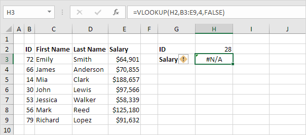
#REF! in cell If col_index_num is higher than the variety of columns in table-array, you'll obtain the #REF! mistake value. For more details on fixing #REF! mistakes in VLOOKUP, see Exactly how to deal with a #REF! mistake. #VALUE! in cell If the table_array is much less than 1, you'll get the #VALUE! error value.

#NAME? in cell The #NAME? error worth generally means that the formula is missing out on quotes. To search for an individual's name, see to it you use quotes around the name in the formula. For example, enter the name as "Fontana" in =VLOOKUP("Fontana", B 2: E 7,2, FALSE). For additional information, see Exactly how to deal with a #NAME! error.

Rumored Buzz on Vlookup For Dummies

Discover exactly how to utilize absolute cell references. Do not save number or date values as text. When searching number or day worths, make sure the information in the first column of table_array isn't kept as message values. Otherwise, VLOOKUP may return an inaccurate or unforeseen worth. Sort the first column Type the initial column of the table_array before making use of VLOOKUP when range_lookup holds true.

An enigma matches any type of solitary character. An asterisk matches any kind of sequence of characters. If you want to discover a real inquiry mark or asterisk, kind a tilde (~) in front of the character. As an example, =VLOOKUP("Fontan?", B 2: E 7,2, FALSE) will look for all instances of Fontana with a last letter that could vary.

When browsing message worths in the initial column, see to it the data in the initial column doesn't have leading rooms, tracking spaces, inconsistent usage of straight (' or") as well as curly (' or ") quote marks, or nonprinting personalities. In these situations, VLOOKUP might return an unforeseen value.

You can always ask a professional in the Excel Individual Voice. Quick Recommendation Card: VLOOKUP refresher Quick Recommendation Card: VLOOKUP fixing tips You Tube: VLOOKUP videos from Excel neighborhood experts Whatever you require to learn about VLOOKUP Exactly how to correct a #VALUE! mistake in the VLOOKUP function Exactly how to fix a #N/ A mistake in the VLOOKUP function Summary of solutions in Excel Exactly how to stay clear of busted formulas Discover errors in formulas Excel functions (indexed) Excel functions (by category) VLOOKUP (free sneak peek).

To compute delivery cost based on weight, you can utilize the VLOOKUP feature. In the instance revealed, the formula in F 8 is: =VLOOKUP(F 7, B 6: C 10,2,1)* F 7 This formula utilizes the weight to locate the appropriate "cost per kg" after that ... To bypass output from VLOOKUP, you can nest VLOOKUP in the IF feature.

how to use vlookup in excel for zip codes vlookup in excel in another sheet vlookup in excel in bengali